An optimality proof of the Muon weight update

This article expects comfort with undergraduate linear algebra. It aims to be explicit and self-contained, with proofs of useful lemmas included in the appendix.

In Jeremy Bernstein’s great post Deriving Muon, he motivates the weight update for the Muon optimizer using a constrained optimization problem. He gives the solution for the optimal weight update, but I wasn’t sure how he arrived at it.

In this post, I provide an optimality proof of the solution. If you’re already familiar with Muon and the constrained optimization problem used to derive its weight update, click here to jump to the proof.

Addendum 2025-07-28: Laker Newhouse pointed out that he and Jeremy also provide a proof of this result in a Dec 2024 paper. See Proposition 5 and its proof in Appendix B. Thanks Laker!

A quick recap of Muon

Define a loss function $\mathcal{L}$. Consider it as a function of the weights of one linear layer, $W$. For a given change in the weights $\Delta W$, the new loss value at $W + \Delta W$ is approximately $$L(W + \Delta W) \approx \mathcal{L}(W) + \langle \nabla_{W} \mathcal{L}, \Delta W \rangle,$$ using the first-order Taylor approximation. Here, the inner product $\langle \cdot, \cdot \rangle$ is the Frobenius inner product on matrices,$$\langle A, B \rangle := \mathrm{Tr}(A^TB).$$Using this Taylor approximation, the change in loss is therefore roughly the inner product $$\mathcal{L}(W + \Delta W) - \mathcal{L}(W) \approx \langle \nabla_{W} \mathcal{L}, \Delta W \rangle.$$ Muon aims to maximize the improvement in loss, subject to a norm constraint on $\Delta W$.

Specifically, it employs the root-mean-square operator norm, $\|\cdot \|_\text{RMS}.$ We’ll properly derive this norm below. But briefly, $\|A\|_{\text{RMS}}$ is the largest possible factor by which a matrix $A \in \mathbb{R}^{m \times n}$ can scale the size of its input, normalized by dimension: $$\|A\|_{\text{RMS}} := \sqrt{ \frac{n}{m} } \text{sup}_{x \neq 0} \frac{\|Ax\|_{2}}{\|x\|_{2}} \tag{1}$$ So we arrive at the constrained optimization problem ($\dagger$) that motivated Muon: $$\text{min} \ \langle \nabla_{W} \mathcal{L}, \Delta W \rangle \quad \text{s.t.} \quad \|\Delta W\|_\text{RMS} \leq \eta. \tag{†}$$ For intuition, the requirement that $\|\Delta W\|_\text{RMS} < \eta$ is equivalent to the condition that the change in the layer’s outputs is bounded by the size of its inputs. From ($1$), $$\|(W + \Delta W)x - Wx \|_{\text{RMS}} = \|(\Delta W)x\|_{\text{RMS}} < \eta \sqrt{ \frac{m}{n} } \|x\|_{\text{2}},$$ for all $x$. So the constraint $\|\Delta W\|_{\text{RMS}} < \eta$ directly ensures that the layer’s outputs don’t change too much within an optimization step.

If we take the singular value decomposition of the gradient as $\nabla_{W} \mathcal{L} = U \Sigma V^T$, then the solution to $(\dagger)$ is given as the “orthogonalization,” $$\Delta W^* = -\eta \sqrt{ \frac{m}{n} } UV^T. \tag{§}$$ In this post, we’ll derive this solution and prove that it is optimal for ($\dagger$). First, some background on the RMS operator norm.

Preliminaries: RMS norm

For an $n$-dimensional vector $x \in \mathbb{R}^{n}$, the RMS norm is defined as $$\|x\|_{\text{RMS}} := \frac{1}{\sqrt{n}} \|x\|_{2} = \sqrt{ \frac{1}{n} \sum_{i = 1}^n x_{i}^{2} }.$$ A useful fact for intuition is that the RMS norm is just the $\ell_2$ norm, rescaled such that the ones vector $\mathbf{1} \in \mathbb{R}^{n}$ has norm $1$ instead of $\sqrt{n}$: $$\|\mathbf{1}\|_{\text{RMS}} = \frac{1}{\sqrt{ n }} \|\mathbf{1}\|_{2} = \frac{1}{\sqrt{n }} \sqrt{ n } = 1.$$ This rescaling allows for a “dimension-invariant” notion of $\ell_2$ size.

We can use this vector norm to define a norm on matrices.

Preliminaries: RMS operator norm

The RMS operator norm is defined to be the largest multiple that a matrix $A$ can increase the RMS norm of its input:$$\|A\|_{\text{RMS}} := \text{sup}_{x \neq 0} \frac{\|Ax\|_{\text{RMS}}}{\|x\|_{\text{RMS}}}.$$ This is trivially equivalent to the definition from $(1)$. Expanding the RMS operator norm using the RMS vector norm definition, $$\|A\|_{\text{RMS}} = \text{sup}_{x \neq 0} \frac{(1 / \sqrt{ m })\|Ax\|_{2}}{(1 / \sqrt{ n })\|x\|_{2}} = \sqrt{\frac{n}{m} } \text{sup}_{x \neq 0} \frac{\|Ax\|_{2}}{\|x\|_2}.$$ The RMS operator norm can also be expressed in terms of the singular values of $A$. For those familiar, the right-hand supremum in the equation above is known as the spectral norm, $$\|A\|_{*} := \text{sup}_{x \neq 0} \frac{\|Ax\|_{2}}{\|x\|_{2}}.$$ The spectral norm of a matrix, the most $A$ can stretch a vector in the $\ell_2$ sense, is precisely its largest singular value: $$\|A\|_{*} = \text{sup}_{x \neq 0} \frac{\|Ax\|_{2}}{\|x\|_{2}} = \sigma_{\text{max}}(A).$$ See Fact 1 for a formal proof. Taking the equality at face value, we now observe, $$\|A\|_{\text{RMS}} = \text{sup}_{x \neq 0} \frac{\|Ax\|_{\text{RMS}}}{\|x\|_{\text{RMS}}} = \sqrt{ \frac{n}{m} } \text{sup}_{x \neq 0} \frac{\|Ax\|_{\text{2}}}{\|x\|_{\text{2}}} = \sqrt{ \frac{n}{m} } \sigma_\text{max}(A). \tag{2}$$ We now have all the machinery we need to solve the Muon problem ($\dagger$). Before we do so, let’s warm up with a simpler problem.

Warmup: Maximizing inner products

Consider the linear program, $$\text{max} \ a^T b \quad \text{s.t.} \quad \|b\|_{2} \leq \alpha.$$ The answer is likely immediately obvious: pick $b$ in the direction of $a$, scaled to the appropriate norm size. Specifically, let $b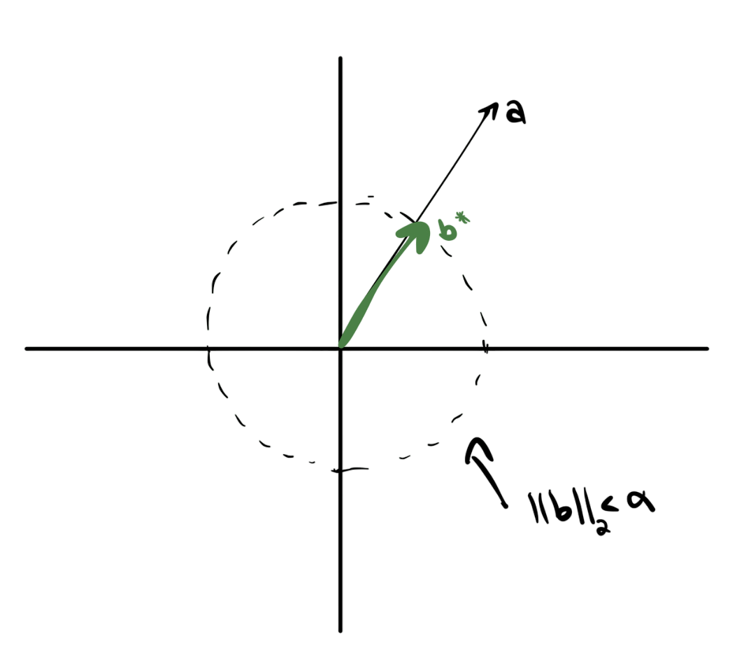$ be $$b = \frac{\alpha}{\|a\|_{2}} a.$$ Picking $b$ to be “aligned with” $a$ to maximize the inner product is pretty intuitive. But how might we prove this?

One option is to assume that we’ve found a better candidate, say $c$, and find a logical contradiction. If we find a contradiction, the better candidate $c$ cannot actually exist—so we win.

Proof: let’s assume that we have $c$ such that $$a^T c > a^T b = \alpha \|a\|_{2}.$$ We want to show that any such $c$ is not a valid solution to our linear program. To do so, we’ll show that it violates the norm condition, meaning $\|c\|_{2} > \alpha.$

We’ll do this using the Cauchy-Schwarz inequality¹. The inequality tells us that $$|a^Tc| \leq \|a\|_{2} \|c\|_{2}.$$ Using our assumption that $a^Tc > a^Tb$, $$\|c\|_{2} \geq \frac{1}{\|a\|_{2}} |a^Tc| > \frac{1}{\|a\|_{2}} |a^Tb| = \frac{1}{\|a\|_{2}} \alpha\|a\|_{2} = \alpha.$$ So $c$ doesn’t satisfy the norm constraint, meaning it is not a valid solution to the problem.

But the only thing we asked of $c$ is that it has a better objective value than $b$. Therefore the same argument applies to all vectors $x$ with $a^Tx > a^T b$. This means that all vectors $x$ with a strictly larger objective value are invalid solutions. In other words, $b$ is optimal.

End proof.

With this, we’re now equipped to analyze the Muon problem.

Back to Muon

The parallels between the warmup problem, $$\text{max} \ a^T b \quad \text{s.t.} \quad \|b\|_{2} \leq \alpha,$$ and the Muon problem ($\dagger$), $$\text{min} \ \langle \nabla_{W} \mathcal{L}, \Delta W \rangle \quad \text{s.t.} \quad \|\Delta W\|_\text{RMS} \leq \eta,$$should be clear. In both cases, we’re optimizing an inner product over a norm ball.

For ease of exposition, we’ll frame the Muon problem ($\dagger$) as a maximization problem in this article. So we’ll instead aim to solve:$$\text{max} \ \langle -\nabla_{W} \mathcal{L}, M \rangle \quad \text{s.t.} \quad \|M\|_{\text{RMS}} \leq \eta. \tag{2}$$ To build intuition for the solution $(\S)$, we’ll first solve a slightly simplified version of the problem in which $\Delta W^*$ will arise naturally.

Then, like the warmup, we’ll proceed by contradiction and show that any candidate better than $\Delta W^*$ does not satisfy the RMS condition.

Why orthogonalize? Deriving a solution a priori

First, the simplified problem.

Based on the warmup, to optimize our inner product objective, we might expect a solution that feels like a matrix “in the direction” of $-\nabla_{W}\mathcal{L}$ . So let’s restrict our attention to matrices $M$ with the same singular basis as $-\nabla_W \mathcal{L}$.

This simplification will allow us to analytically derive the optimal weight update $\Delta W^*$.

Reducing to the same singular basis

Since $\nabla_{W} \mathcal{L} = U\Sigma V^T$, a valid SVD of the negative gradient is simply $$-\nabla_{W} \mathcal{L} = -(U\Sigma V^T) = (-U)\Sigma V^T$$ So take $M$ to be a matrix $$M = (-U) D V^T,$$ for some arbitrary nonnegative diagonal matrix $D$.

Writing out the objective value, we have $$\langle -\nabla_{W} \mathcal{L}, M \rangle = \Big\langle (-U)\Sigma V^T, (-U)DV^T \Big\rangle.$$ It turns out that the Frobenius inner product does not change when you pre- or post-multiply by orthogonal matrices (Fact 2). So $$\langle -\nabla_{W} \mathcal{L}, M \rangle = \Big\langle (-U)\Sigma V^T, (-U)DV^T \Big\rangle = \langle \Sigma, D \rangle.$$ Since $\Sigma$ is a diagonal matrix, we can write the matrix inner product as a function only of the diagonal entries of each matrix: $$\langle \Sigma, D \rangle = \mathrm{Tr}(\Sigma^T D) = \sum_{i} \Sigma_{ii} D_{ii}.$$ We can simplify this expression even further. If we pull out the diagonal elements into vectors, defining $\sigma := \text{vec}(\Sigma)$ and $d := \text{vec}(D)$, we can rewrite the sum as $$\langle -\nabla_{W} \mathcal{L}, M \rangle = \sum_{i} \Sigma_{ii} D_{ii} = \sum_{i} \sigma_{i} d_{i} = \sigma^T d.$$ We’ve now reduced the matrix inner product objective to a vector inner product.

We can also express the $\mathrm{RMS}$ norm of $M$ in terms of $d$. Since the entries of $d$ are the singular values of $M$ by construction, we have that $$\|M\|_{\text{RMS}} = \sqrt{ \frac{n}{m} } \text{max}_{i} d_{i},$$by equation $1$.

In our restricted setting, then, we’ve now successfully reduced the matrix-domain problem ($\dagger$) to the vector-domain problem, $$\text{max} \ \sigma^T d \quad \mathrm{s.t.} \quad \text{max}_{i} \ d_{i}\leq \eta\sqrt{ \frac{m}{n} }.$$ This reduced version is quite easy to solve.

Deriving a solution

Since $\sigma$ represents the singular values of $-\nabla_W \mathcal{L}$, it must have nonnegative elements. So maximizing the inner product $\sigma^T d$ is equivalent to maximizing each of the component products $\sigma_i d_i$.

Under our constraint on $d_i$, then, the best solution to this reduced problem is simply the constant vector $$d_{i} := \eta \sqrt{ \frac{m}{n} }.$$ If this isn’t immediately obvious, try to prove it yourself.

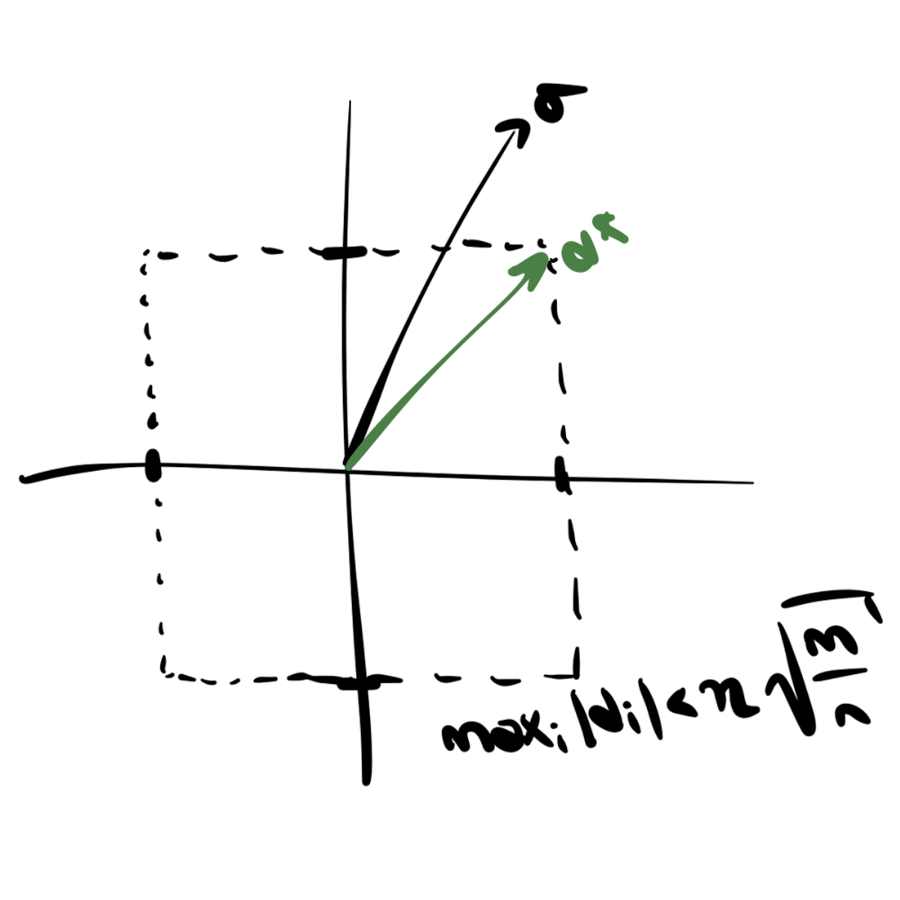
Translating from the vector parameter $d$ to the matrix parameter $M$, the best solution to our restricted matrix-domain problem is therefore $$M = (-U)DV^T = (-U)(d_{i}I)V^T = -\eta \sqrt{ \frac{m}{n} }UV^T.$$This is precisely the optimal value ($\S$) given by Bernstein!

It’s now clearer why it’s a good idea to define our weight update as the negative gradient $-\nabla_{W} \mathcal{L}$ with its singular values “clamped” to $\eta \sqrt{ m / n }$.

For a weight update $M$ in the same singular basis as $-\nabla_{W}\mathcal{L}$, the inner product objective and the RMS norm are expressible entirely in terms of the singular values of $-\nabla_{W} \mathcal{L}$ and $M$. The inner product objective turns into a dot product between two nonnegative singular value vectors $\sigma, d$. And the RMS norm constraint turns into an element-wise maximum constraint on the singular values $d$ of $M$. The optimal solution is therefore just to clamp the parameters $d$ to their maximum allowable values.

Just like the warmup problem, then, the solution is a “rescaled” (singular value clamped) matrix $M$ “in the direction of” (in the same singular basis as) the negative gradient $-\nabla_{W} \mathcal{L}$.

With this intuition, we can dive into the proof.

A proof of optimality

The proof is not as elegant as the warmup, since we can’t use Cauchy-Schwarz.² But it relies on the same contradiction technique.

Assume we have some matrix $A$ that does better than $\Delta W^*$, meaning $$\langle -\nabla_{W} \mathcal{L}, A \rangle > \langle - \nabla_{W}\mathcal{L}, \Delta W^* \rangle. \tag{3}$$We’ll show that $\|A \|_\text{RMS} > \eta$ and therefore that $A$ cannot be a solution to $(\dagger)$.

Proof: First, we’ll rewrite $A$ in terms of the singular basis $-U, V$ as $$A = (-U)BV^T,$$ defining $B = (-U)^T A V$. With this, we can simplify the problem expression slightly.

Using the fact that the Frobenius inner product is invariant under orthogonal transformations of its inputs (Fact 2), we can rewrite the objective as: $$\langle -\nabla_{W} \mathcal{L}, A \rangle = \big\langle (-U)\Sigma V^T, (-U)BV^T \big\rangle = \langle \Sigma, B \rangle.$$ Since $\Sigma$ is diagonal, this reduces to $$\langle \Sigma, B \rangle = \mathrm{Tr}(\Sigma^TB) = \sum_{i} \Sigma_{ii} B_{ii}.$$ Applying the same argument to $\Delta W^*$, we have $$\langle -\nabla_{W} \mathcal{L}, \Delta W^* \rangle = \Big\langle \Sigma, \left(\eta \sqrt{ m / n } \right) I \Big\rangle = \sum_{i} \Sigma_{ii} \left( \eta \sqrt{ \frac{m}{n} } \right).$$ Our assumption in $3$ means that $$\langle -\nabla_{W} \mathcal{L}, A \rangle - \langle - \nabla_{W}\mathcal{L}, \Delta W^* \rangle > 0.$$ So $$\sum_{i} \Sigma_{ii} \left( B_{ii} - \eta \sqrt{ m / n } \right) > 0.$$ For this sum to be strictly positive, at least one term must be strictly positive. Call this term $i$. All singular values are nonnegative, so $\Sigma_{ii} \geq 0$. For the $i$th term in the sum to be positive, then, we must have $$B_{ii} > \eta \sqrt{ m / n }. \tag{4}$$This fact will be the key to showing $\|A\|_\text{RMS} > \eta$.

By Fact 3, the RMS norm is invariant under orthogonal transformations, so $$\|A\|_\text{RMS} = \|B\|_{\text{RMS}}.$$ It therefore suffices to show $\|B\|_\text{RMS} > \eta.$ To do this, all we need to do is find one vector $v$ such that $$\|Bv\|_{\text{RMS}} > \eta\|v\|_{\text{RMS}}. \tag{5}$$ Pick $v$ to be the $i$th coordinate vector, meaning $$v_{j} = \begin{cases} 1 & j = i \\ 0 & \mathrm{otherwise.} \end{cases}$$ Note that $v$ has unit $\ell_2$ norm, so $$\|v\|_{\text{RMS}} = \frac{1}{\sqrt{ n }} \|v\|_{2} = \frac{1}{\sqrt{ n }}.$$ So $Bv$ is just the $i$th column of $B$, meaning $$(Bv)_{j} = B_{ij}.$$ In particular, $(Bv)_i = B_{ii}.$ Now, we can calculate $\|Bv\|_2$ and attempt to show ($5$). $$\|Bv\|_{2}^{2} = v^T B^T Bv = \sum_{j} B_{ij}^{2} \geq B_{ii}^{2},$$since all other terms in the sum are nonnegative: $B_{ij}^{2} \geq 0$. But from equation $(4)$, we therefore have that $$\|Bv\|_{2} \geq B_{ii} > \eta \sqrt{ m / n }.$$ Applying this inequality to the RMS norm, we find $$\|Bv\|_{\text{RMS}} = \frac{1}{\sqrt{ m }} \|Bv\|_{2} > \frac{1}{\sqrt{ m }} \eta \sqrt{ \frac{m}{n} } = \eta \frac{1}{\sqrt{ n }} = \eta\|v\|_{\text{RMS}}.$$ Therefore $\|B\|_\text{RMS} = \|A\|_{\text{RMS}} > \eta$. So $A$ cannot be a valid solution to the problem, and $\Delta W^*$ as given in Equation ($\S$) is optimal.

End proof.

Conclusion

In this article, we explored and proved the optimality of the solution $\Delta W^*$ to the Muon constrained optimization problem ($\dagger$). We situated it within the framework of maximizing an inner product over a norm ball, and used this analogy to motivate the otherwise potentially-unintuitive formula.

---

Appendix: Useful Facts

Fact 1

The spectral norm of a matrix is its largest singular value.

For any matrix $A \in \mathbb{R}^{m \times n}$, $$\|A\|_{*} = \sigma_{\text{max}}(A),$$ where $\sigma_\text{max}(A)$ is the largest singular value of $A$.

Proof: Let $U \Sigma V^T$ be the SVD of $A$. Without loss of generality, assume the singular values are ordered in descending magnitude, so $\Sigma_{11} \geq \Sigma_{22} \geq \dots$.

To prove the equality, it suffices to prove the inequalities $$\sigma_{\text{max}}(A) \leq \|A\|_{*} \quad \text{and} \quad \|A\|_{*} \leq \sigma_{\text{max}}(A).$$ We’ll start with the left hand inequality.

Step 1: Maximum Singular Value $\leq$ Spectral Norm

To show this, it suffices to find some vector $v$ such that $$\|Av\|_{2} / \|v\|_{2} = \sigma_{\text{max}}(A).$$ But this is trivial. Let $v := Ve_1$, where $e_1$ is the coordinate vector with first component $1$ and all other components $0$. Then $$Av = U\Sigma V^T (Ve_{1}) = U \Sigma e_{1} = U(\sigma_{\text{max}}(A)e_{1}) = \sigma_{\text{max}}(A) Ue_{1}.$$ Taking norms, I claim that $\|v\|_2 = \|Ue_1\|_2 = \|e_1\|_2 = 1$, where the middle equality follows because orthogonal matrices preserve $\ell_2$ norms. The proof of this claim is simple. Let $O$ be an orthogonal transformation and $w$ an arbitrary vector. Then $$\|Ow\|_{2}^{2} = w^T O^TOw = w^T I w = w^T w = \|w\|_{2}^{2}.$$ And so $\|Ue_1\|_2 = \|e_1\|_2 = 1$. Therefore, we’ve found a vector $v$ such that $$\frac{\|Av\|_{2}}{\|v\|_{2}} = \|Av\|_{2} = \sigma_\text{max}(A)\|Ue_{1}\| = \sigma_{\text{max}}(A).$$ So the spectral norm must be at least the maximum singular value, $$\|A\|_{*} \geq \sigma_{\text{max}}(A).$$

Step 2: Spectral Norm $\leq$ Maximum Singular Value

For this inequality, we need to show that $$\|Av\|_{2} \leq \sigma_{\text{max}}(A) \|v\|_{2}$$ for all vectors $v \in \mathbb{R}^{n}$.

Again relying on the fact that orthogonal matrices preserve the $\ell_2$ norm, Therefore $\|Av\|_2$ = $\| \Sigma V^T v\|_2$. Define $w := V^T v$, so $$\|Av \|_{2} = \|\Sigma w\|_{2}.$$

Each element of $\Sigma w$ is just $(\Sigma w)_i = \Sigma_{ii} w_i$. And each diagonal element $\Sigma_{ii}$ is bounded by the maximum singular value, $\sigma_\text{max}(A)$. So $$(\Sigma w)_{i} = \Sigma_{ii} w_{i} \leq \sigma_{\text{max}}(A) w_{i},$$ And therefore $$\|\Sigma w\|_{2} \leq \sigma_{\text{max}} \|w\|_{2}$$ But $w = V^Tv$ and $V$ is orthogonal, so $\|w\|_{2} = \|v\|_{2}$. We conclude, $$\|Av\|_{2} = \|\Sigma w\|_{2} \leq \sigma_{\text{max}} \|w\|_{2} = \sigma_{\text{max}}\|v\|_{2}.$$ End proof.

Fact 2

The Frobenius inner product is invariant under orthogonal transformations.

Let $A$ and $B$ be arbitrary $m \times n$ matrices. And let $U \in \mathbb{R}^{m \times m}, V \in \mathbb{R}^{n \times n}$ be orthogonal matrices, meaning $$U^TU = UU^T = I_{m} \quad \text{and} \quad V^TV = VV^T = I_{n}.$$ Then $$\langle UAV^T, UBV^T \rangle = \langle A, B \rangle$$ Proof: Expand out the definition of the Frobenius inner product, $$\begin{align*} \langle UAV^T, UBV^T \rangle &= \mathrm{Tr} \Big( (UAV^T)^T (UBV^T) \Big) \\ &= \mathrm{Tr} ( VA^T (U^TU) BV^T) \\ &= \mathrm{Tr} (VA^T BV^T). \end{align*}$$Using the cyclic trace property³, this reduces to $$\mathrm{Tr}(V A^T B V^T) = \mathrm{Tr}(A^T B V^T V) = \mathrm{Tr}(A^TB) = \langle A, B \rangle.$$ End proof.

Fact 3

The RMS norm is invariant under orthogonal transformations.

Let $A$ be an $m \times n$ matrix, and let $U \in \mathbb{R}^{m \times m}, V \in \mathbb{R}^{n \times n}$ be orthogonal. Then $$\|A\|_{\text{RMS}} = \|UAV^T \|_{\text{RMS}}.$$ Proof: For brevity, call $B := UAV^T$. Since $$\| M \|_{\text{RMS}} = \sqrt{ \frac{n}{m} } \sigma_{\text{max}}(M),$$ it suffices to show that $B$ and $A$ have the same singular values.

Say $A = LSR^T$ is the SVD of $A$. Without loss of generality, order the singular values in descending magnitude, so $$S_{11} \geq S_{22} \geq \dots$$ So we can write $B$ as $$B = U A V^T = (UL) S (RV)^T.$$ But since $U, L, R, V$ are all orthogonal matrices, the above is a SVD of $B$. So the two matrices have the same maximum singular value, $$\sigma_{\text{max}}(A) = \Sigma_{11} = \sigma_{\text{max}}(B).$$ Therefore $$\|A\|_{\text{RMS}} = \sqrt{ \frac{n}{m} } \sigma_{\text{max}}(A) = \sqrt{ \frac{n}{m} } \sigma_{\text{max}}(B) = \|B\|_{\text{RMS}}.$$ End proof.

---